< Continued from Page 4
Continued on Page 6 >
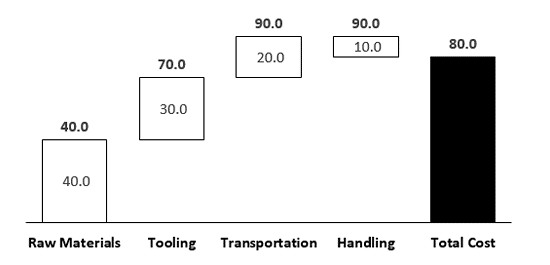
Now that you know how to build a Waterfall chart with positive numbers, the question is how to you handle negative numbers? Although this requires a bit more work, it’s no problem if you keep your spreadsheet organized.
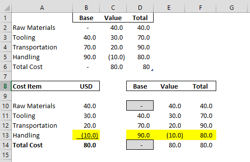
Negative Waterfall Scenario: Continuing with the same example, if we change the handling fee above from a positive 10 to a negative 10 (a handling discount), the Excel spreadsheet updates to a total cost of 80 (I’ve marked the row in yellow within Figure 1), below.

Figure 1: Excel Sheet Handling Discount of 10
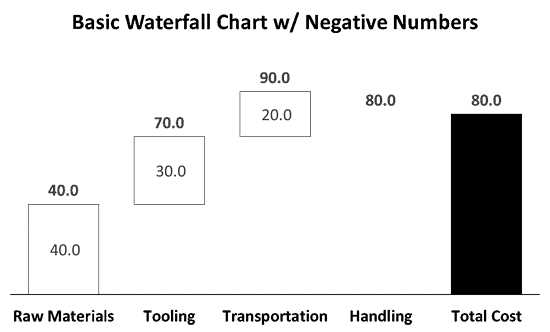
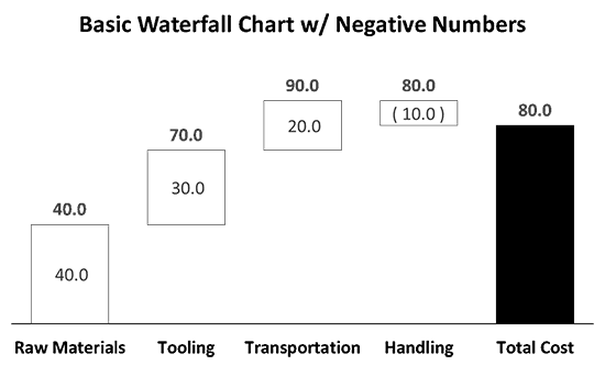
With the handling discount of 10, the Waterfall Chart in PowerPoint is no longer correct as the Handling column disappears, as can be seen in Figure 2), below.

Figure 2: PowerPoint Resulting Waterfall Chart
Follow these steps to resolve this issue:
- Fix the Base: First you'll need to navigate back to the Excel spreadsheet. Right-click your chart and select the Edit in Excel option to return to the Excel spreadsheet.
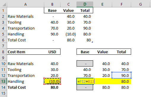
- For rows with negative numbers, marked in yellow in the spreadsheet, the Base will need to adjust due to the negative number. So in cell D13, change the formula to "=F12 + B13", which takes the Base of the Handling column down to 80.

Figure 3: Adjusting the Base Formula in Excel 
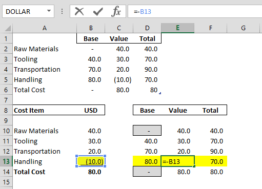
Figure 4: Resulting Waterfall Chart in PowerPoint - Fix the Value: To bring the Value column back into our PowerPoint chart, we need to change the negative value of 10, to a positive value, while still keeping our data dynamic. So instead of hard-coding it in, in cell E13 simply change the formula to "=-B13". Reversing the sign creates a positive value, which brings the column back into our PowerPoint chart, as you can see on the right of Figure 5. Now we’ll just need to manually adjust the label.

Figure 5: Adjusting the Label Formula in Excel 
Figure 6: Resulting Waterfall Chart in PowerPoint after fixing values - Fixing the Data Label in PowerPoint: To close Excel, hit Ctrl + W on your keyboard to return to PowerPoint. Now that we have manually adjusted the formulas in Excel, we need to manually adjust the Data Label for the negative value within the Waterfall Chart itself.
- To do so, double-click into the Handling Data Label, and wrap parentheses around the number to indicate that it is negative. If you want, you can also fill the Handling column's Value column with another color, to further indicate that it’s a negative number.

Figure 7: Wrap parentheses around the number Note: If at any point your number changes back to positive value, you will need to go back into Excel to adjust the formulas, and then correct the data label manually back in PowerPoint.
- Spot Checking: Even though all the numbers are correct, it’s a best practice to visually spot check your Waterfall Chart for accuracy to make sure the items are adding up and subtracting correctly.
Ending Excel Spreadsheet Formulas for your Negative Waterfall Chart
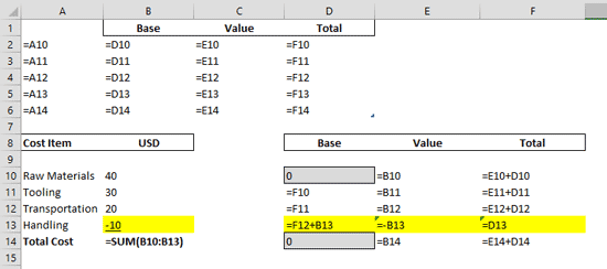
Just as a reference, below is what the formulas inside the Excel spreadsheet should look like for your negative Waterfall Chart.

Figure 8: Formulas inside the Excel spreadsheet
Waterfall Chart Additions – Adding Step Lines, continued on Page 6 >
