Create a Waterfall Chart in PowerPoint - Part 4

< Continued from Page 3

Continued on Page 5 >

Formatting the Column Chart:

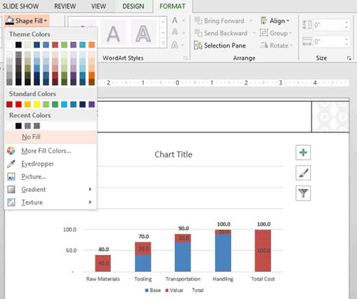
1. Hiding the Total Columns: With the Data Labels now all set up correctly, the next step is to hide the columns that we don't want to see, starting with the Total columns. So right-click the green series, so that all of the green columns are selected, and from the Chart Tools Format Tab in the Ribbon, select the No Fill option, which for all intents and purposes, makes the green series disappear (see Figure 1 below).
2. 
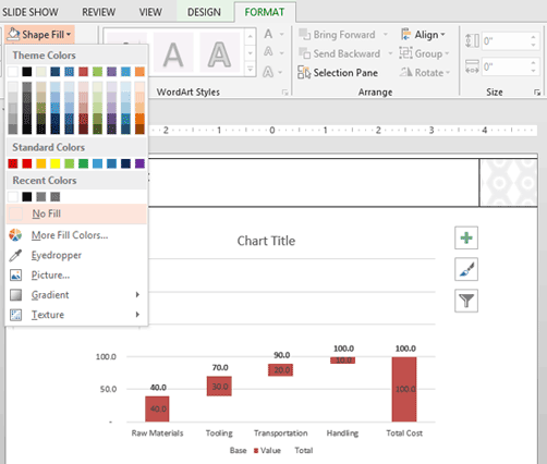
   Figure 1: Chart Tools Format tab - Green Series
2. Hiding the Base Columns: Next, let's do the same with the Base columns. Right-click the blue series, so that all of the blue columns are selected, and from the Chart Tools Format tab, select the No Fill option, which for all intents and purposes, makes the blue series disappear (see Figure 2 below).
3. 
   Figure 2: Resulting formatted Blue Series
3. Changing the Formatting of the Value column: Next let's change the Value column to a white fill with a black outline. Right-click the red series, so that all of the red columns are selected, and from the Chart Tools Format tab, change the fill to white and the outline to black (see Figure 3 below).
4. 
   Figure 3: Resulting Waterfall Chart

Adjusting the Chart's Dimensions

Now you can clearly see the Waterfall chart. From here we can make some aesthetic adjustments to improve the visual quality of the chart.

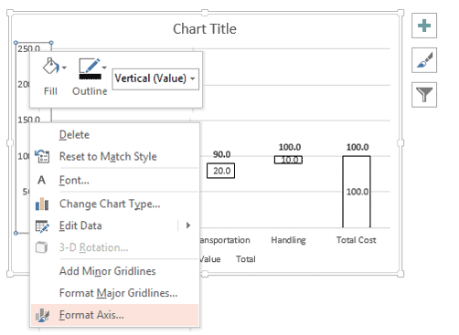
1. Adjusting the Vertical Axis: To get rid of all the blank space, we need to adjust the vertical axis. Right-click the vertical axis on the left, and select Format Axis option (see Figure 4 below).
2. 
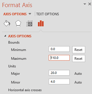
   Figure 4: Formatting the Vertical Axis
3. Within the Format Axis Task Pane that opens (see Figure 5 below), you can now manually hard code in a minimum value of 0 and a maximum value of 110 (so that the Task Pane brings up the Reset button next to the numbers) and then close the Task Pane.
4. 
   Figure 5: Hard Coded Min and Max Values
Note: If you are using different numbers from this example, simply input the minimum and maximum values that fit your data range.
2. Cleaning up the Chart: To further clean up the aesthetics of the chart, from here I would recommend the following adjustments:
• Remove the Vertical Axis: Select the vertical axis on the left and hit Delete.
• Remove the Final Data Label: Select the final data label within the Final Total column, in this example it's 100, and hit Delete.
• Format the Total Cost Column: Select the final column in the Waterfall Chart and fill it black (or some other solid color), to indicate that it is different from the other pieces of the Waterfall Chart.
• Remove the Gridlines: Select the gridlines and hit Delete.
• Remove the Legend: Select the legend at the bottom at hit Delete.
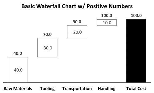
• Format the Chart’s Title: Format the Chart Title by making it black and size 24, and replace "Chart Title" with the title of your chart, in this example it's "Basic Waterfall Chart w/ Positive Numbers."
• Format the Total Column’s Data Labels: Change the Total column's data labels to size 18.
• Format the Value Column's Data Labels: Change the Value column's data labels to size 14.
• Format the X-Axis: Change the X-Axis line to black with a 1 PT weight, and make the font size of the X-Axis labels size 18 (how big you make them will affect how large your chart is).
• Change the Column Gap Width: Right-click the series and in the Format Series dialog box, change the column Gap Width to 50%.
3. 
   Figure 6: Pre-Formatted Chart
4. 
   Figure 7: Post-Formatted Chart

Ending Excel Spreadsheet Formulas for your Waterfall Chart

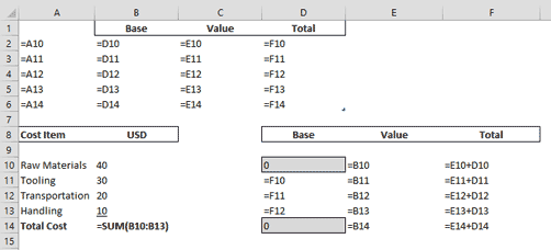
Just as a reference, below is what the formulas inside the Excel spreadsheet of your Waterfall chart should look like.

And keep in mind that we wrote dynamic formulas for cells A2 through D6, so that they are only referencing the Base, Value, and Total calculations in the cells below (see Figure 8 below). With the whole spreadsheet dynamic like this, updating your chart is a cinch: Simply update your numbers in cells B10 through B13 and the rest of the spreadsheet updates automatically!

Figure 8: Excel Spreadsheet Formulas for Waterfall Chart

Waterfall Chart Additions - Working with Negative Numbers, continued on Page 5 >