The data labels that you add to your PowerPoint charts can be enhanced by exploring Format Data Label options. These Format Data Label options include Label Options to edit the content, the position, and the format of data labels, as explained in this tutorial.
To begin, you need to have a chart on your slide. If you don't have one, insert a chart on your slide. Thereafter, enable data labels for your chart.
Then, follow these steps to format data labels in PowerPoint 2013 for Windows:
- Bring up the Format Data Labels Task Pane as explained in Step 1 within our Format Data Label Options for Charts in PowerPoint 2013 for Windows tutorial. Thereafter proceed with these further steps.
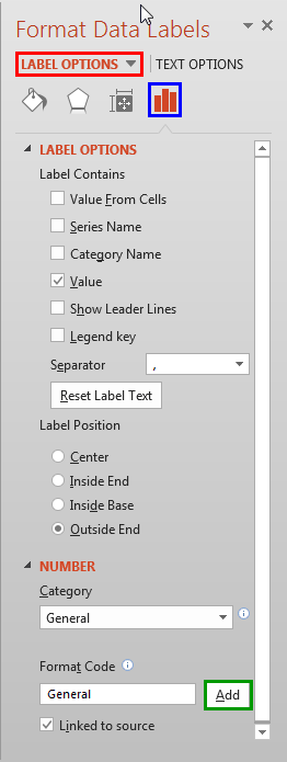
- In this Task Pane, make sure that the Label Options tab, as shown highlighted in red within Figure 1, below is selected. Then, click the Label Options button, as shown highlighted in blue within Figure 1.

Figure 1: Label Options within Format Data Labels Task Pane - As you can see in Figure 1 above, Label Options have been divided into two categories: Label Options and Number. Let us start with exploring options within the Label Options section:
Label Contains
- Includes check-boxes that decide the content of data labels. These are:
Value From Cells
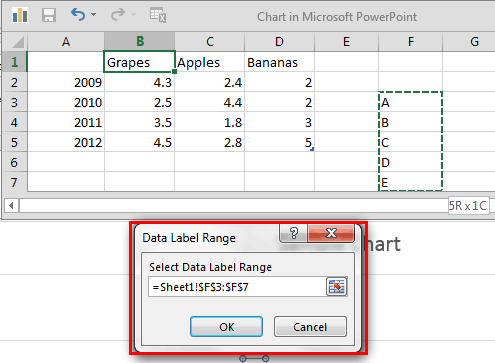
- This option is useful when you have stored labels or values you want to show as part of the data label, in an Excel sheet within a set of adjacent cells. This check-box may not be available if you have selected only one data label. To use this option, first make sure you keep the Excel sheet containing the data labels open before you select this check-box. Selecting this check-box launches an instance of Excel sheet, along with Data Label Range dialog box as shown highlighted in red within Figure 2, below.

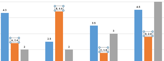
Figure 2: Data Label Range dialog box - Within the instance of the open Excel sheet, select the set of adjacent cells that contain text or digits that you want to show as part of the data label. Take a look at the instance of Excel sheet in our sample chart within Figure 2, above, where we have selected cells containing alphabets A to E. The selection is also reflected within the Data Label Range dialog box. Click the OK button when you are done to see the result within the chart's data labels, as shown in Figure 3, below.

Figure 3: Alphabets taken from Excel cells added as part of the data label Series Name
- Displays name of the series in data labels.
Category Name
- Displays name of the category in data labels.
Value
- Displays data values of series in data labels.
Show Leader Lines
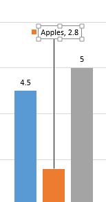
- Select to show the leader lines. A leader Line is a line that points to a data label to its associated data point (or, column in a column chart). This option is helpful when you’ve placed a data label away from a data point (or column).

Figure 4: Leader Line Legend key
- Select this check-box if you want to show the legend key (the color block shown in chart legends) in front of the data label. Figure 4, above shows the legend key in front of the data label.
Label Position
- Includes four radio buttons that decide the position of data labels. These options have already been explained in our Chart Data Labels in PowerPoint 2013 tutorial.
- Now, let's explore options within the Number section:
Category
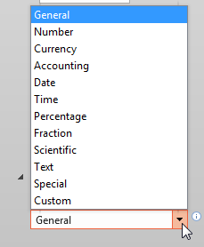
- Clicking this option opens a drop-down menu as shown in Figure 5, below. Click on the required format option for the data labels to select it.

Figure 5: Category drop-down list Format Code
- This option is helpful when you want your data labels to be easily-readable. This is done by changing longer digits to show fewer digits. To do so, first you need to select the Custom option within the Category drop-down list. Then, within the Format Code box, type the required format of the data label numbers to be displayed. Thereafter, click the Add button,highlighted in green within Figure 1, as shown previously on this page, to apply the new format.
- Use any of the Label Options to format your data labels as required.
- Save your presentation often.
